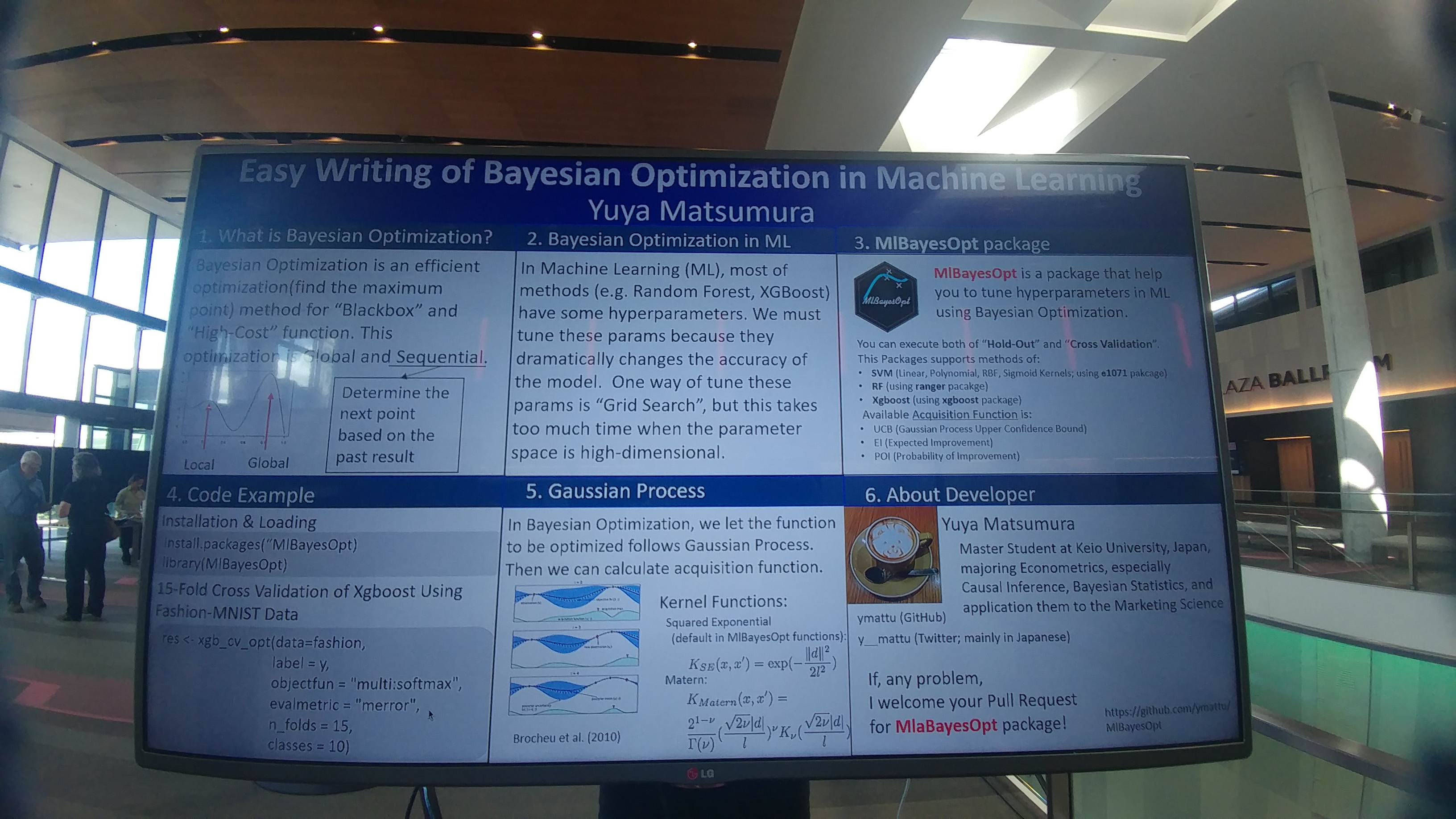
Easy Writing for Bayesian Optimization in Machine Learning
MlBayesOpt package
@y__mattu
Tokyo.R #71
July 15, 2018
Introduction
Profile
- Yuya MATSUMURA
(松村優哉) - Twitter: y__mattu
- GitHub: ymattu
- Graduate student of Keio University
- Studying: Econometrics, Bayesian Statistics, Causal Inference
- Languages: R, Python, SAS
![]()
useR!2018
Fantastic Conference

hexwall

Poster Presentation

Today’s Talk:
In short…
- Very short summary of poster presentation at useR!2018
- cf. Global TokyoR #2
- Today’s content is updated.
Summary of this package
About this package
- MlBayesOpt(https://github.com/ymattu/MlBayesOpt)
- This package make it easier to write a script to execute parameter tuning using bayesian optimization.
- SVM(Linear, Polynomial, RBF, Sigmoid Kernels)、Random Forest、XGboost
- Based on following packages:
- SVM(e1071)
- RF(ranger)
- XGboost(xgboost)
- Bayesian Optimization(rBayesianOptimization)
- Wecan use both of “Hold-Out” and “Cross Validation”
MlBayesOpt
Installation and Loading
Installation
install.packages("MlBayesOpt")
devtools::install_github("ymattu/MlBayesOpt")
Loading
library(MlBayesOpt)Usage
Hold-Out
SVM
set.seed(123)

res0 <- svm_opt(train_data = iris_train,
                train_label = Species,
                test_data = iris_test,
                test_label = Species,
                svm_kernel = "polynomial",
                init_points = 10,
                n_iter = 1)
Output of SVM (Excerpt)
elapsed = 0.01  Round = 1   degree_opt = 5.0000 coef0_opt = 1.2641  Value = 0.9333
elapsed = 0.01  Round = 2   degree_opt = 7.0000 coef0_opt = 7.6410  Value = 0.9333
elapsed = 0.01  Round = 3   degree_opt = 5.0000 coef0_opt = 1.5038  Value = 0.9600
elapsed = 0.01  Round = 4   degree_opt = 4.0000 coef0_opt = 7.6924  Value = 0.9333
elapsed = 0.01  Round = 5   degree_opt = 5.0000 coef0_opt = 8.4372  Value = 0.9333
elapsed = 0.01  Round = 6   degree_opt = 10.0000    coef0_opt = 7.7898  Value = 0.9333
elapsed = 0.01  Round = 7   degree_opt = 8.0000 coef0_opt = 1.4249  Value = 0.9200
elapsed = 0.01  Round = 8   degree_opt = 9.0000 coef0_opt = 8.0788  Value = 0.9333
elapsed = 0.01  Round = 9   degree_opt = 5.0000 coef0_opt = 8.9781  Value = 0.9333
elapsed = 0.01  Round = 10  degree_opt = 6.0000 coef0_opt = 9.2771  Value = 0.9333
elapsed = 0.01  Round = 11  degree_opt = 10.0000    coef0_opt = 4.4448  Value = 0.9333

Best Parameters Found:
Round = 3   degree_opt = 5.0000 coef0_opt = 1.5038  Value = 0.9600
Cross Validation
SVM
set.seed(71)
res0 <- svm_cv_opt(data = iris,
                   label = Species,
                   n_folds = 3,
                   init_points = 10,
                   n_iter = 1)
Output of SVM
elapsed = 0.02  Round = 1   gamma_opt = 3.3299  cost_opt = 11.7670  Value = 0.9333
elapsed = 0.01  Round = 2   gamma_opt = 5.5515  cost_opt = 76.1740  Value = 0.9067
elapsed = 0.01  Round = 3   gamma_opt = 3.2744  cost_opt = 14.1882  Value = 0.9400
elapsed = 0.01  Round = 4   gamma_opt = 2.1175  cost_opt = 76.6932  Value = 0.9200
elapsed = 0.01  Round = 5   gamma_opt = 3.1619  cost_opt = 84.2154  Value = 0.9600
elapsed = 0.01  Round = 6   gamma_opt = 9.4727  cost_opt = 77.6772  Value = 0.8933
elapsed = 0.01  Round = 7   gamma_opt = 6.6175  cost_opt = 13.3914  Value = 0.9267
elapsed = 0.02  Round = 8   gamma_opt = 8.8943  cost_opt = 80.5955  Value = 0.8733
elapsed = 0.01  Round = 9   gamma_opt = 3.3808  cost_opt = 89.6793  Value = 0.9333
elapsed = 0.01  Round = 10  gamma_opt = 4.3481  cost_opt = 92.6987  Value = 0.9000
elapsed = 0.01  Round = 11  gamma_opt = 2.9508  cost_opt = 84.8600  Value = 0.9467

Best Parameters Found:
Round = 5   gamma_opt = 3.1619  cost_opt = 84.2154  Value = 0.9600
XGboost
set.seed(71)

res0 <- xgb_cv_opt(data = iris,
                   label = Species,
                   objectfun = "multi:softmax",
                   evalmetric = "mlogloss",
                   n_folds = 3,
                   classes = 3,
                   init_points = 2,
                   n_iter = 1)
)
About arguments
ex. “Hold Out” using SVM
res <- svm_opt(
  # about dataset (at least required)
  train_data = iris_train,
  train_label = Species,
  test_data = iris_test,
  test_label = Species,
  # about hyper parameters (optional, default is following)
  svm_kernel = "radial", # RBF
  gamma_range = c(10 ^ (-5), 10 ^ 5),
  cost_range = c(10 ^ (-2), 10 ^ 2),
  # about bayesian optimization (optional, default is following)
  init_points = 20,
  n_iter = 1,
  acq = "ei",
  kappa = 2.576,
  eps = 0.0,
  optkernel = list(type = "exponential", power = 2)
  )
Future Works
This package is still a development version…
- Fix some bugs
- Make functuions about Deep Learning…? (mxnet package…?)
Enjoy R programming !
This slide is made from revealjs package.
This slide and Rmd file are published on Git Hub(https://github.com/ymattu/TokyoR71).